The Natural Rate of Interest.
Explored Interactively.
Decompose the forces driving real interest rates in advanced economies, explore supply-demand non-linearities, and build custom scenarios with our heterogeneous-agent general equilibrium life-cycle model.
See It in Action
Dashboard Preview
Explore seven interactive views spanning baseline projections, decomposition, supply-demand diagrams, scenarios, and real-world market comparisons. Country-specific analysis coming shortly.
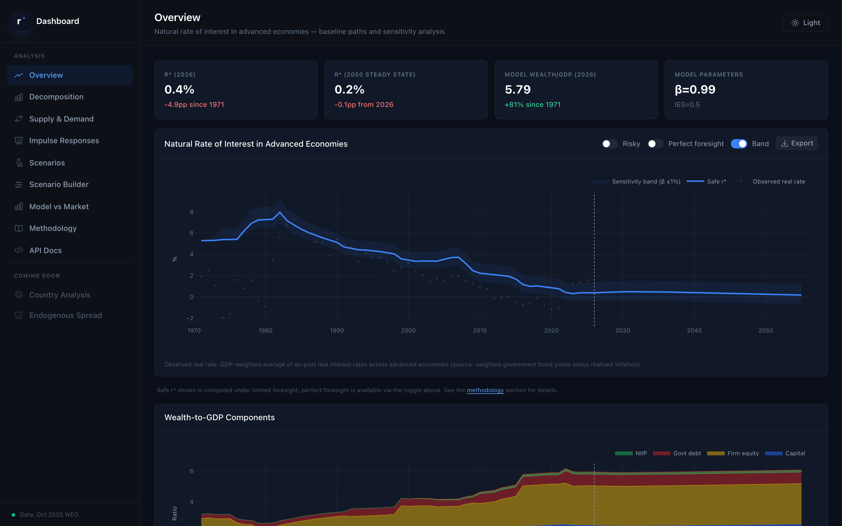
Overview
Track r* from 1970 to 2055 with sensitivity bands
Features
Comprehensive r* Analysis Tools
Baseline r* Paths
Track the natural rate from 1970 to 2055 under perfect and limited foresight, with sensitivity bands.
Force Decomposition
Isolate the contribution of 15 structural forces — demographics, TFP, fiscal policy, and more.
Supply-Demand Diagrams
Visualize asset market equilibrium: how demand and supply curves shift to determine r*.
Scenario Analysis
Compare 6 pre-built scenarios: deglobalization, AI boom, fiscal expansion, and more.
Custom Scenario Builder
Drag sliders to create your own macro scenarios and see r* respond in real-time.
Country-Level Analysis
Explore r* paths for 7 major economies with country-specific calibrations.
Workflow
Embed r* in Your Investment Process
No macro strategy should exist without being stress-tested against a structural model of interest rates.
Build Custom Scenarios
Drag 12 sliders to construct your macro view — from AI-driven productivity booms to fiscal expansions. See exactly how each force moves r* and download the results.
Open Scenario BuilderExport & Integrate
Download scenario data as CSV or JSON, or hit our API endpoints directly. Plug r* projections into your models, dashboards, and risk systems.
View API DocsDecompose What Drives Rates
Isolate the contribution of each structural force — demographics, fiscal policy, technology, global savings. Understand why rates moved and where they're heading.
View DecompositionMethodology
General Equilibrium Model of Advanced Economies
Overview
The dashboard is built on an overlapping-generations (OLG) life-cycle model in which heterogeneous agents save for retirement, invest in risky capital, and hold safe government bonds. The natural rate of interest r* is determined in capital market equilibrium — where the demand for assets (from firms, the government, and the rest of the world) equals the supply (accumulated household wealth).
The model is calibrated to match the macroeconomic experience of advanced economies from 1970 to the present and is continuously updated with new data and methodological improvements. It incorporates 15 exogenous driving forces: demographics (population growth, retirement length, working-life duration), technology (TFP growth, depreciation, capital share), fiscal policy (government debt, spending, social security, taxes, military spending), markups, risk premia, and global capital flows.
Limited Foresight vs Perfect Foresight
The model can be solved under two alternative information assumptions about how agents form expectations regarding future changes in the economic environment.
Perfect Foresight (PF)
Agents are assumed to know the entire future sequence of shocks from the moment they arrive at the current period. They anticipate all future changes in demographics, productivity, fiscal policy, and other forces, and optimize their saving and investment decisions accordingly. This is the standard rational expectations benchmark.
Limited Foresight (LF)
Agents have only limited foresight of what is coming. They are surprised periodically by larger shifts in the economic environment — formally, each shift is treated as an unexpected (MIT) shock. After each shift, agents believe the economy will remain at the new steady state forever, until the next surprise arrives. This “episodic updating” captures the idea that agents do not fully anticipate slow-moving structural changes.
Quantitatively, the limited foresight path for r* is around 0.5–0.7 percentage points lower than the perfect foresight path today. The baseline results shown in the dashboard use the limited foresight solution.
Supply and Demand for Assets
Capital demand D(r) is the total demand for assets in the economy: physical capital K, capitalized firm profits Π, and government debt B. Each component falls as the interest rate rises, so the aggregate demand curve is downward-sloping and convex.
Capital supply S(r) is the long-run capital supply schedule — it shows how much wealth households accumulate at each interest rate in steady state.
Decomposition
The force decomposition isolates the contribution of each structural force to the change in r* by computing the equilibrium interest rate that would prevail if only that single force had changed from its 1970 value to its current/projected value, holding all other forces constant. The total change is then the sum of all individual contributions.
Reference
Rachel, Lukasz (2025). “What Next for r*? A Capital Market Equilibrium Perspective on the Natural Rate of Interest.”
Brookings Papers on Economic Activity, Fall 2025.
The dashboard model is based on the framework developed in this paper but is continuously improved with new data, updated calibrations, and methodological enhancements.
Read the full paperInstitutional Access
Built for Investment Professionals
Whether you run a macro fund, advise a central bank, or allocate a pension portfolio — understanding the structural anchor for interest rates is essential. The r* dashboard gives you a model-based framework grounded in peer-reviewed research, updated quarterly with new data.
What’s included
- Full dashboard access with all analytical tools
- Custom scenario builder with real-time r* projections
- Quarterly data updates with new WEO and demographic vintages
- Country-level calibrations (coming soon)
- Data export and API access
- Downloadable scenario data (CSV/JSON) and programmatic API access for integration into your own systems
- Direct briefings from the model author
Or contact Lukasz Rachel directly to arrange a demo.